12 Google Sheet Formulas to Simplify Your SEO Data Management

Data skills form the backbone of all keyword selection, content optimisation, competitive analysis, and tracking for digital marketing SEOs. Data allows us to identify content gaps and opportunities, compare against competitors, and measure performance. And the more granular your categorisation and data filtering, the more efficient and quickly you can develop your SEO strategy. Better insights, better recommendations, and voila, everyone’s happy!

However, data filtering and analysis can be a laborious and time-consuming task. That’s particularly true with the data sets that SEOs manage, which is why so many often turn to SEO tools to help them get the job done. However, there are plenty of cheaper and equally efficient Google Sheets formulas to help you manage data, create dashboards, or build analysis templates. Here are some of our favourite hacks in a step-by-step guide to save you time on your SEO tasks.

Psssst: We built a live Google sheet for all the formulas mentioned that you can use to practice or better understand the formulas in action better.

Quick Links:

Filtering Data in Google Sheets

Categorising Data in Google Sheets

Analysing Data in Google Sheets

H2: What data management skills does an SEO need?

I usually tackle these 4 SEO tasks daily:

Filtering junk data from large data sets
Data Categorisation
Data Reporting: Using Graphs or Pivot Tables
Data Analysis: Where are the patterns and recommendations behind them?

Google Sheet filtering data hacks: Removing irrelevant keywords

Data filtering is critical for SEO keyword research as it ensures accuracy, relevance, and efficiency in your data set. It also helps guarantee you are sticking with correct geographical targeting, language considerations, and niche specificity. As always though it can be hard to figure out which part of the data is relevant and if not, how to bulk delete irrelevant terms. So here are a few of my favourite case study scenarios when it comes to filtering out data sets.

Removing place names

When I’m looking at a large e-commerce website, and not local SEO, place names I find in keyword data are typically not important to begin with. That’s why I like to use IF and REGEXMATCH—it cuts the task of removing them down.

Enter a list of place names between the | | in the following formula:

This will let you know in a separate column whether there is a place name (of the ones you entered in the formula) in the keywords. This should make it easy to use the filter function to select all the keywords returning “UK place names found” and bulk delete.

You can adapt the place names to be any you like but to save time, I often use ChatGPT to build the list with the top UK cities by population. You can also manually input locations where you know your offering is irrelevant. (Be careful not to add too many as there is a character limit for Google Sheets formulas.)

This may not be a hard-and-fast, completely-eradicates-all hack, but it should help reduce your filtering time.

Removing brand terms

Regarding e-commerce sites, you can make some of the biggest SEO gains with non-brand keywords, mostly because this is where you can often find juicy search volume.

I find the easiest way to do this is to exclude common brand names from a data search in Semrush or Ahrefs before you even begin to pull your data.

Excluding brand terms from a keyword list using Semrush

Semrush has an exclude branded keywords tool that looks like this:

However, I find its track record of actually removing branded terms is patchy at best.

Excluding brand terms when pulling data from Ahrefs

Create a long list of brand names that are separated by commas (e.g CSV) for your chosen sector and input them into the ‘Exclude Keyword’ tab before you export. It may look something like this:

To generate the list you can type into ChatGPT:

“Give me a list of brands in the haircare space in a CSV list provide all you can think of and please include common misspellings”

Then enter it into Ahrefs before exporting data.

Again, you may still miss some brands when you export your data for manual filtering, but it should cut down on a huge bulk of junk data you don’t need to focus on.

Removing brand names when they already exist in your data

Already downloaded the keyword list with data? No problem, you can use that catchy hack I mentioned earlier to REGEXMATCH for them:

=IF(OR(REGEXMATCH(A2, “\b(brand1|brand2|brand3|brand4|)\b”)), “Brand names found”, “No Brand Names found”)

As with before, use the filter function to select all the keywords that include brand names and bulk delete.

Removing misspellings in a list of keywords

While there isn’t a specific formula in Google Sheets to automatically correct misspellings in keyword data, you can utilise certain functions and techniques to help identify and clean up misspelt keywords.

Use Spell Check

Google Sheets provides a built-in spell-checking feature to help you identify misspelt keywords. Select the data range containing the keywords, go to the “Tools” menu, and choose “Spelling.” The spell checker will highlight any potential misspellings, allowing you to review and correct them manually.

Using a Fuzzy Lookup (VLOOKUP or INDEX-MATCH)

You can use the fuzzy lookup approach to identify and correct misspellings by comparing keywords against a reference list. Create a reference list of correctly spelt keywords in a separate sheet or column. Then, use functions like VLOOKUP or INDEX-MATCH with approximate matching to compare and find the closest match for each keyword.

Filtering out foreign language terms in Google Sheets

If you’re working in an English-only market, foreign language terms will not be relevant to your analysis. For this scenario, the formula is relatively straightforward. Add another column next to your keyword data and plug in the following Google Sheets formula:

=DETECTLANGUAGE(A1)

Semrush has a language filter you can use to filter out before you export any keywords into lists. However, the results may vary because it is in BETA.

You can use it for an initial pass and then do another sweep of your data in Google Sheets for this scenario.

This should let you know where in the data it detects non-English terms. Now this formula isn’t 100% accurate, so it may be best to scan by filtered views of the languages quickly.

Google Sheets formulas for categorising data

Categorising your keyword research data is a vital part of noticing patterns and gaps in your SEO coverage. For many digital marketers, this is where you’ll first notice the recommendations you need in your content marketing strategy.

Using a keyword clusterizer add-on

Some wonderful SEOs at Variant Marketing have helped tackle this issue by creating a Keyword Clusterizer you can run as a Google Sheets add-on in your file. I personally love this for smaller data sets as it helps find lexical groups in your data so you can start noticing patterns straight away.

Just download it to Chrome, run it through your Google Sheets file as an add-on, and watch the magic happen as it allows you to click hot or cold depending on if you find your data relevant or not.

Using Google Sheets REGEXMATCH to categorise your data

If you’re pulling keywords from competitors or your own sites where a URL will be tied to a keyword, using regex can be a great way to notice which subfolders on your or a competitor’s site are ranking well, and which subfolders need more constructive SEO graft for your client.

Regular expressions (regex) identify patterns in a string, allowing you to extract specific parts. To extract a subfolder name from a URL, regex then finds and captures the desired pattern for extraction. For example,

You have a URL ranking for the keyword “childrens curtains”, which subfolder is it ranking for?

Let’s take an example URL to demonstrate,

The URL: https://www.therange.co.uk/furnishings/bedding/childrens-bedding/childrens-curtains/

The formula:

=REGEXEXTRACT(E2, “/furnishings/([^/]+)/”)

This will pull in the subfolder after furnishings, in this case,

“bedding”.

So imagine the formula like this:

=REGEXEXTRACT(E2, “/the folder before the one you want to pull/([^/]+)/”)

This will then allow you to see what sort of categories are ranking for a large volume of keywords using a Pivot Table or SumIF Function. (more about those later)

Using Apps script to create your own formulas for data reviewing

Google Apps Script may seem complicated at first, but with the right tools, it can help you create custom-built scripts (or code) that will give you custom formulas for analysing data in Google Sheets.

What is Apps Script?

Google’s Apps Script is a platform that makes it fast and easy to write code in modern JavaScript and has access to built-in libraries for Google Workspace applications like Gmail, Calendar, Sheets, and more. What this means in terms of Google Sheets is that you can run custom code to run your own custom formulas. And the best part is that you don’t have to be a coding whizz to give it a go if you have ChatGPT at your fingertips.

How to use Apps Script in Google Sheets

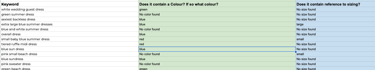
You can query ChatGPT to provide an APPs script for your dilemma. For Example:

“can you write me an apps script for if a keyword contains a reference to sizes for example, medium, large, extra small, small and so on?”

It can then spit out a javascript that looks something like this:

/**
* Checks if a cell value contains a reference to sizes and returns the mentioned size.
*
* @param {string} text – The text to check for size references.
* @return {string} The mentioned size or “No size found”.
* @customfunction
*/
function getSizeFromText(text) {
  var sizes = [“extra small”, “small”, “medium”, “large”, “extra large”];
  text = text.toLowerCase();
  for (var i = 0; i < sizes.length; i++) {
    if (text.indexOf(sizes[i]) !== -1) {
      return sizes[i];
    }
  }
  return “No size found”;
}

Click ‘extensions’, run the Apps script, and copy and paste. Once saved, it should provide you with a custom Google sheets formula. In the case of the one above, ChatGPT has named it:

=getSizeFromText(A1)

Input this into an additional column and select the cell you want it to analyse.

For example

I have created a similar one in the example Google Sheet, so have a play around and see if you can create some custom functions for yourself.

3 Google Sheets formulas for data analysis

Now that we know exactly what keywords we want to focus on and we won’t be pestered by any bizarre characters, foreign languages, or irrelevant and annoying brand terms, we can now start analysing the data.

What is it that is helping your competitor to rank better for a term? How can you replicate that for yourself?

ImportXML

ImportXML is a fantastic function to use if you want to observe the differences in meta-data that may be helping the top SERP competitors rank better for specific terms.

Let’s say you’ve noticed from your gap analysis that your site only ranks on the 2nd page for the keyword “Formal Dresses” and you want to get in on those top 3 positions in SERPs. Well, using ImportXML allows you to import various structured data types including XML, HTML, CSV, TSV and RSS and Atom XML feeds.

Pulling in meta titles

Just pull the list of URLs in the top of SERPS, add a column for Title and Description and add this formula:

=IMPORTXML(CompetitorURL,”//meta[starts-with(@property, ‘og:title’)]/@content”)

Pulling in meta descriptions

=ImportXML(CompetitorURL,“//meta[@name=’description’]/@content”)

Pulling in H1s, H2s, and H3s

=ImportXML(CompetitorURL, “//h1”)

=ImportXML(CompetitorURL, “//h2”)

=ImportXML(CompetitorURL, “//h3”)

Pulling in all the links on a page

=ImportXML(CompetitorURL, “//@href”)

If you want to play around more with these functions, this specific tab in the aforementioned Google Sheets companion spreadsheet displays all of these formulas.

Some more ImportXML functions for marketers:

All links on a page: “//@href”
Extract all internal links on a page: “//a[contains(@href, ‘example.com’)]/@href”

Analysing Metadata with LEN

The LEN function helps analyse metadata for SEO purposes by calculating the text length within a cell. By using LEN, you can assess the character count of meta titles, descriptions, or other relevant elements to ensure they meet optimal length guidelines for search engine visibility and user experience.

The formula should look something like this:

=LEN(K3)

You can then measure the length of your meta titles and meta descriptions. Remember The ideal length for the meta title is 50–60 characters and the ideal length for a meta description is 150-160 characters.

Visualising trends with Sparkline

Do you want to confirm the trends in a keyword position quickly? Use Sparkline. For example, let’s say you regularly track 150 keywords in a relevant category to your site. For those, you check what position you fall in each month. How do we see the trend over time?

=SPARKLINE(A2:B2)

Using pivot tables to measure SEO metrics

A pivot table is one of the easiest ways to analyse large data sets. In particular, for content gaps, it can show you which areas of your site need more content. You can also see what’s doing well by ranking keywords or by aggregate search volume of keywords.

To create one, click ‘insert’ and then click ‘pivot table’

You can start to notice patterns in your keyword, Google Search Console, and Google Analytics data instantly.

Using Conditional Formatting

Conditional formatting can help you identify trends based on the assigned colours visually. As digital marketers, this enables you to spot patterns, compare data points, and gain insights into the performance of keywords or metrics over time in a snap.

I often use it when performing comparative content audits to identify core issues in content; for example, content with high impressions but low clicks and therefore a very low CTR.

To use conditional formatting, follow these three simple steps:

Select the data range you want to analyse in your Google Sheets. This could be a column or row of SEO data, like keyword rankings or Google search console metrics.
Go to the “Format” menu and choose “Conditional formatting” and then select “Colour scale.” This option allows you to assign different colours to the data based on its relative values.
Now you can set the colour scale rules. In the conditional formatting dialogue box, customise the rules based on the trends you want to focus on.
1. For example, you can choose a green-to-red colour scale, where higher values are shown as greener and lower values as redder. This visual representation helps you identify positive or negative trends in your SEO data.

Importing data using APIs in Google Sheets

Sometimes, you may just need more data to understand what SEO optimisations to make. When this happens, importing additional data using APIs in Google Sheets offers a valuable opportunity to gain deeper insights. APIs for powerful tools, such as Supermetrics or AHREFS, can automate the process and eliminate manual data entry.

Thankfully, Google Sheets provides built-in functions like “IMPORTDATA” and “IMPORTJSON” for streamlined API integration. Input the API endpoint URL, and the data will flow directly into designated cells, saving precious time and effort.

Using VLOOKUP in Google Sheets

Suppose you want to pull that API data into the Google Sheets tab where your other data is against a keyword (for example). In that case, We can use the VLOOKUP function we mentioned earlier again here as it searches for a value in a specified column and returns a corresponding value from the same row.

Let’s say you want to add an extra column for the keyword search console data into your original tab. You know the keyword appears in both tabs, so you can search to find the exact data set for that keyword and pull it into the existing tab to match.

The Formula will look something like this:

=VLOOKUP(A:A,A:C,2,FALSE)

For the more advanced Google Sheets goers, you can add an IFERROR function to make the data returns neater.

=IFERROR(VLOOKUP(A:A,A:C,2,FALSE),”-”)

And there are many, many more

This barely scratches the surface of the number of available functions in Google Sheets, but we hope you’ve found the following tutorial a good place to start.